The Census Reporter was created to make it easier for journalists to write stories using census data. To that end, they’ve created a really slick and easy to use web site that makes the data accessible and fun to explore. From the homepage you have three ways of diving into the data: you can pull up a profile by typing in the name of a place, you can enter an address and explore places that contain that address, or you can explore tables by topic.

First, the place-based approach. You can type in a named place, like a state, county, or a census place (incorporated cities and towns, or census designated places) to get started. This will give you a selection of data from the most recent release of the American Community Survey. For larger areas where the data is available, it gives you 1-year ACS data by default; otherwise you get the latest 5-year data.

You’re presented with a map of the location at the top, and a series of attractive looking graphs and charts sorted by the demographic profile table source – social, economic, housing, and demographic. If you hover over a data point in a table it gives you some geographic context by comparing this place’s value with that of larger places where it’s contained. For example, if I search for Philadelphia I can hover over the chart to get the value for the Philly metro area and the State of Pennsylvania. I can click a link below each chart to open the full table, which includes both estimates and margins of error. There are small links for viewing the table by itself on a separate page (which also gives you the ability to download it) and for embedding the chart in a website.

Viewing the table gives you additional options, like adding additional places for comparison, or subdividing the place into smaller areas for comparison. So if I’m looking at Philadelphia, I can break it down into tracts, block groups, or ZIP Codes. From there I can toggle away from the table view to view a map or a distribution bar to explore that variable by individual geographies.

The place-based search is great at allowing you to drill down either by topic or by these smaller geographies. But if you wanted to access a fuller range of geographies like congressional districts or PUMAs, it seems easier to do an address-based search. Back on the homepage, selecting the address button and typing in an address brings you to a map with the address pin-pointed, and on the left you can choose any geography that encloses that address. Once you do that, you get a profile for that geography and can start doing the same sorts of operations for changing the topics or tables, or adding or subdividing geographies for comparison.

The topic-based search lets you search just by topic and then figure out the geography piece later. Of the three types of searches this one is the toughest, given the sheer number of tables and cross-tabulations. You can click on a link for a general topic to narrow things down a bit before beginning a search.

In downloading the data you have a variety of useful options: CSV, Excel, GeoJSON, KML, and shapefiles. So in theory you can download data that’s readily mappable – in practice I wasn’t able to download a shapefile, but could grab a KML or GeoJson and was able to visualize it in QGIS. One challenge in downloading any of the files is that the column names use the identifier codes, and the actual names of the variables aren’t included in the download format you choose – they’re included in a json file. So you can use that for reference, but it can’t be readily incorporated into the table.

So – where would this resource fall within the pantheon of US Census data resources? I think it’s great for accessing and, especially, visualizing profiles (profile = lots of data for one place) from the most recent ACS releases. It’s easy to use and succeeds at making the data interesting; for that reason I certainly would incorporate it into undergraduate courses where I’m introducing data. The ability to embed the charts into websites is certainly a bonus, and they deserve a big thumbs up for incorporating the margin of error data, rather than hiding or discarding it like other resources do.

The ability to create and view comparison tables (comparison = one piece of data for many places) is good – select an area and then break it down – but not as strong as the profile options. If you want to get a profile for a non-named place like a tract, ZIP Code, or PUMA you can’t do that from the profile search. You can do an address search and back out (if you know an address for that you’re interested in) or you can drill down by topic, which lets you search by summary area in addition to named places.

For users who need to download a lot of data, or for folks who need datasets that aren’t the most recent ACS release, this resource isn’t the place to go. The focus here is on providing the data in an easy and compelling way, as is. In viewing the profiles, it’s not clear if you can choose 5-year data over 1-year data for places where both datasets are available – even for large geographic areas with high population, sometimes it’s preferable to use the 5-year data to take advantage of the smaller margins of error. I also didn’t see an option for choosing decennial census data.

In short, this resource is well-designed and definitely worth exploring. It seems clear why this would be a go-to source for journalists, but it can be for many others as well.

The NYC Department of City Planning has been collating census data and publishing it for the City for quite some time. They’ve created neighborhood tabulation areas (NTAs) by aggregating census tracts, so that they could publish more reliable ACS data for small areas (since the margins of error for census tracts can be quite large) and so that New Yorkers have data for neighborhood-like areas that they would recognize. The City also publishes PUMA-level data that’s associated with the City’s Community Districts, as well as borough and city-level data. All of this information is available in a large series of Excel spreadsheets or PDFs in the form of comparison tables for each dataset.

The Department of Planning also created the NYC Census Factfinder, a web-mapping interface that let’s users explore census tract and NTA level data profiles. You could plug in an address or click on the map and get a 2010 Census profile, or a demographic change profile that showed shifts between the 2000 and 2010 Census.

It was a nice application, but they’ve just made a series of updates that make it infinitely better:

1. They’ve added the American Community Survey data from 2009-2013, and you can view the four demographic profile tables (demographics, social, economic, and housing) for tracts and NTAs.
2. Unlike many other sources, they do publish the margin of error for all of the ACS data, which is immensely important. Estimates that have a high margin of error (as defined by a coefficient of variation) appear in grey instead of solid black. While the actual margins are not shown by default, you can simply click the Show radio button to turn on the Reliability data.
3. Tracts or neighborhoods can be compared to the City as a whole or to an individual borough by selecting the drop down for the column header.
4. This is especially cool – if you’re viewing census tracts you can use the select pointer and hold down the Control key (Command key on a Mac) to select multiple tracts, and then the data tables will aggregate the tract-level data for you (so essentially you can build your own neighborhoods). What’s noteworthy here is that it also calculates the new margins of error for all of the derived estimates, AND it even calculates new medians and averages with margins of error! This is something that I’ve never seen in any other application.
5. In addition to searching for locations by address, you can hit the search type drop down and you have a number of additional options like Intersection, Place of Interest, and even Subway Stations.

There are a few quirks:

1. I had trouble viewing the map in Firefox – this isn’t a consistent problem but something I noticed today when I went exploring. Hopefully something temporary that will be corrected. Had no problems in IE.
2. If you want to click to select an area on the map, you have to hit the select button first (the arrow beside the zoom slider and print button) and then click on your area to select it. Just clicking on the map without hitting select first won’t do much – it will just highlight the area and tell you it’s name. Clicking the arrow button turns it blue and allows you to select features, clicking it again turns it white and lets you identify features and pan around the map.



3. The one bummer is that there isn’t a way to download any of the profiles – particularly the ones you custom design by selecting tracts. Hitting the Get Data button takes you out of the Factfinder and back to the page with all of the pre-compiled comparison tables. You can print the table out to a PDF for presentation purposes, but if you want a data-friendly format you’ll have to highlight and select the table on the page, copy, and paste into a spreadsheet.

These are just small quibbles that I’m sure will eventually be addressed. As is stands, with the addition of the ACS and the new features they’ve added, I’ll definitely be integrating the NYC Census Factfinder into my presentations and will be revising my NYC Neighborhood Census data handout to add it as a source. It’s unique among resources in that it provides NTA-level data in addition to tract data, has 2000 and 2010 historical change and the latest 5-year ACS (with margins of error) in one application, and allows you to build your own neighborhoods to aggregate tract data WITH new margins of error for all derived estimates. It’s well-suited for users who want basic Census demographic profiles for neighborhood-like areas in NYC.

I kept searching for some definitive proof, and through someone’s tweet I found a link to a PDF of the US Census Bureau’s Budget Estimates for Fiscal Year 2016, presented to Congress this February 2015. I found confirmation buried on page CEN – 106 (the 100th page in a 190 page doc):

Data Products

Restoration of ACS Data Products ($1.5 million): Each year, the ACS releases a wide range of data products widely used by policymakers, Federal, state and local governments, businesses and the public to make decisions on allocation of taxpayer-funds, the location of businesses and the placement of products, emergency management plans, and a host of other matters. Resource constraints have led to the cancellation of data products for areas with populations between 20 and 60 thousand based on 3-year rolling averages of ACS data (known as the “3-Year Data” Product).They have also resulted in delays in the release of the 1- and 5- year Public Use Macro Sample (PUMS) data files and canceled the release of the 5- year Comparison Profile data product and the Spanish Translation of the 1- and 5- year Puerto Rico data products.

The Census Bureau proposes to terminate permanently the 3-Year Data Product. The Census Bureau intended to produce this data product for a few years when the ACS was a new survey. Now that the ACS has collected data for nearly a decade, this product can be discontinued without serious impacts on the availability of the estimates for these communities.

The ACS would like to restore the timely release of the other essential products in FY2016. The continued absence of these data products will impact the availability of data – especially for Puerto Rico – to public and private sector decision makers.

So at this point it’s still just a proposal. The benefits, besides the ability to release other datasets in a timely fashion, would be simplification for users. Instead of choosing between three datasets now there will only be two – the one year and the five year. You choose the one year for large areas and the five year for every place else. In terms of disadvantages, consider this example – here are the number of children enrolled in nursery school in NY State PUMA 03808, which covers Murray Hill, Gramercy, and Stuyvesant Town in the eastern half of Midtown Manhattan:

Population Over 3 Years Old Enrolled in Nursery / Pre-school

• 1 year 2013: 1,166 +/- 609
• 3 year 2011-2013: 1,549 +/- 530
• 5 year 2009-2013: 1,819 +/- 409

Since PUMAs are statistical areas built to contain 100k people, data for all of them is available in each series. Like all the ACS estimates these have a 90% confidence interval. Look at the data for the 1-year series. The margin of error (ME) is so large that’s it’s approximately 50% of the estimate, which in my opinion makes it worthless for just about any application. The estimate itself is much lower than the estimate for the other two series. It’s true that it’s only capturing the latest year, but administrative data and news reports suggest that the number of nursery school children in the district that covers this area has been relatively stable over time, with modest increases (geographically the district covers an area much larger than this PUMA). This suggests that the estimate itself is not so great.

The 5 year estimate may be closer to reality, and its ME is only 20% of the estimate. But it covers five years in time. If you wanted something that was a compromise – more timely than the five year but with a lower ME than the one year, then the three year series was your choice, in this case with an ME that’s about 33% of the estimate. But under this proposal, this choice goes away and you have to make do with either 1-year estimates (which will be lousy for geographies that aren’t far above the 65k population threshold, and lousy for small population groups where ever they are located), or better 5-year estimates that cover a greater time span.

Loading shapefiles can be done via the pgAdmin III GUI (for this example, used version 1.18 for MS Windows) from a client machine using the shp2pgsql-gui. This is an extra plugin that must be downloaded and installed. A command line version of the tool (shp2pgsql) is automatically bundled with PostGIS, but can’t be used by a client unless they either log into the server via a terminal or install PostGIS locally.

Download Plugin

The shp2pgsql-gui can be downloaded for MS Windows from the extras folder on the PostGIS website: http://download.osgeo.org/postgis/windows/. Version 2.01 for 32 bit environment was downloaded and unzipped. Per the instructions in the README file, the postgisgui folder was dragged into the PG BIN path as designated in pgAdmin under File > Options > Binary Paths. Once pgAdmin was restarted the gui was available under the Plugins menu.

Load Shapefiles

Set Options

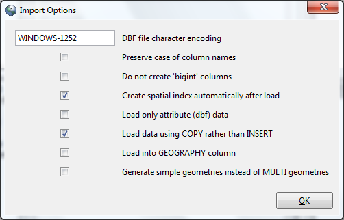
Under Plugins > PostGIS Shapefile and DBF Loader, Check the Options Menu. There are often problems when dealing with UTF-8 encoding in DBF files and when working in an MS Windows environment. Change encoding from UTF-8 to WINDOWS-1252 (another possibility would be LATIN-1). Keep boxes for creating spatial index and using COPY instead of INSERT checked.

Load

Browse and select both shapefiles. Once they appear in the import list the following elements must be changed: switch schema from public to desired schema (usa_general), change table to give each one a meaningful name, and specify the SRID number for each (since these files are from the US Census they’re in NAD 83, which is EPSG 4269). Once you hit Load, the log window will display the results of each import.

Refresh the database and both shapefiles will appear as tables.

Check Geometries

Because of the size of some geometries, they may appear blank if you preview the tables in pgAdmin – this is a well known and documented issue. The simplest way to verify is to check and make sure that none of the geometry columns are null:

SELECT COUNT(*)
FROM usa_general.states
WHERE geom IS NULL;

“0”

Post-Load Operations

Primary Keys

By default, PostGIS will automatically create a field called gid using sequential integers, and will designate this field as the primary key. If the data already has a natural key that you want to use, you would have to drop the key constraint on gid and add the constraint to the desired field. Since features from the US Census have unique ANSI / FIPS codes, we’ll designate that as the key.

ALTER TABLE usa_general.states
DROP CONSTRAINT states_pkey

Query returned successfully with no result in 125 ms.

ALTER TABLE usa_general.states
ADD CONSTRAINT states_pkey PRIMARY KEY (“state”);

Query returned successfully with no result in 125 ms.

Constraints

An alternative to changing the primary key would be to add UNIQUE and NOT NULL constraints to additional columns; gid remains as the primary key but the other columns will automatically be indexed when constraints are added.

ALTER TABLE usa_general.metros ADD CONSTRAINT cbsa_unq UNIQUE (cbsa);
ALTER TABLE usa_general.metros ALTER COLUMN cbsa SET NOT NULL;

Delete Records

For sake of example, we’ll delete all the records for micropolitan areas in the metros table, so we’re left with just metropolitan areas.

DELETE FROM usa_general.metros
WHERE lsad=’Micro’

Query returned successfully: 581 rows affected, 219 ms execution time.

Spatial SQL

As a test we can do a query to select all of the populated places that are within the NYC metropolitan area but are not in Pennsylvania, that have an elevation greater than or equal to 500 feet.

SELECT feature_name, state_alpha, county_name, elev_in_ft
FROM usa_general.pop_places, usa_general.metros
WHERE metros.cbsa=’35620′
AND ST_WITHIN(pop_places.geom, metros.geom)
AND elev_in_ft >= 500
AND state_alpha !=’PA’
ORDER BY elev_in_ft DESC

“Kampe”;”NJ”;”Sussex”;1293
“Highland Lakes”;”NJ”;”Sussex”;1283
“Edison”;”NJ”;”Sussex”;1234″…

Connect to QGIS

We can look at the geographic features by establishing a connection between the database and QGIS. In QGIS we can either hit the add PostGIS Layer button or use the browser to connect to a our database; we need to add the connection name, host, port, and database name. The username and password can be left blank and Q will prompt the user for it (if you don’t want it saved on the system). Once the connection is established you can add the layers to the view and change the symbolization.

• The Social Explorer: this web-mapping resource for depicting and accessing US Census data from 1790 to present (including the 2010 Census and the latest American Community Survey data) is intuitive and user-friendly. Many academic and public libraries subscribe to the premium edition that provides full access to all features and datasets (so check with yours to see if you have access), while a basic free version is available online. Given the current circumstances the Social Explorer team has announced that it will open the hatch and provide free access to users who request it.
• The NHGIS (National Historic GIS): this project is managed by the Minnesota Population Center and also provides access to all US Census data from 1790 to present. While it’s a little more complex than the Social Exlorer, the NHGIS is the better option for downloading lots of data en-masse, and is the go-to place if you need access to all datasets in their entirety, including all the detail from the American Community Survey (as the Social Explorer does not include margins of error for any of the ACS estimates) or if you need access to other datasets like the County Business Patterns. Lastly – it is the alternative to the TIGER site for GIS users who need shapefiles of census geography. You have to register to use NHGIS, but it’s free. For users who need microdata (decennial census, ACS, Current Population Survey), you can visit a related MPC project to the NHGIS: IPUMS.
• The Missouri Census Data Center (MCDC): I’ve mentioned a number of their tools in the past; they provide easy-to-access profiles from the 2010 Census and American Community Survey, as well as historical trend reports for the ACS. For intermediate users they provide extract applications for the 2010 Census and ACS for creating spreadsheets and SAS files for download, and for advanced users the Dexter tool for downloading data en-masse from 1980 to present. Unlike the other resources no registration or sign-up is required. I also recommend the MCDC’s ACS and 2010 Census profiles to web designers and web mappers; if you’ve created online resources that tapped directly into the American Factfinder via deep links (like I did), you can use the MCDC’s profiles as an alternative. The links to their profiles are persistent and use a logical syntax (as it looks like there’s no end in site to this shutdown I may make the change-over this week). Lastly, the MCDC is a great resource for technical documentation about geography and datasets.
• State and local government: thankfully many state and local governments have taken subsets of census data of interest to people in their areas and have recompiled and republished it on the web. These past few weeks I’ve been constantly sending students to the NYC Department of City Planning’s population resources. Take a look at your state data center’s resources, as well as local county or city planning departments, transportation agencies, or economic development offices to see what they provide.

The article is available via Emerald’s journal database. If you don’t have access to it from your library feel free to contact me and I’ll send you a copy (can’t share this one freely online).

Title: The American Community Survey: practical considerations for researchers
Author(s): Francis P. Donnelly
Citation: Francis P. Donnelly, (2013) “The American Community Survey: practical considerations for researchers”, Reference Services Review, Vol. 41 Iss: 2, pp.280 – 297
Keywords: American Community Survey, Census, Census geography, Data handling, Decennial census, Demographic data, Government data processing, Government information, Margins of error, Sample-based data, United States of America, US Census Bureau
Article type: Technical paper
DOI: 10.1108/00907321311326228 (Permanent URL)
Publisher: Emerald Group Publishing Limited

The Census FTP site at http://www2.census.gov/

This would be the first logical step, but in the end it wasn’t optimal based on my need. When you drill down through Census 2010, Summary File 1, you see a file for every state and a national file. Initially I thought – great! I’ll just grab the national file. But the national file does NOT contain the small census statistical areas – no tracts, block groups, or blocks. If you want those small areas you have to download the files for each of the states – 51 downloads. When you download the data you can also download an MS Access database, which is an empty shell with the geography and field headers, and you can import each of the text file data tables (there a lot of them for 2010 SF1) into the db and match them to the headers during import (the instructions that were included for doing this were pretty good). This is great if you need every variable in every table for every geography, but I was only interested in one table for one geography. I could just import the one text file with my table, but then I’d have to do this import process 51 times. The alternative is to use some Python to get that one text file for every state into one big file and then do the import once, but I opted for a different route.

The NHGIS at https://www.nhgis.org/

I always recommend this resource to anyone who’s looking for historical census data or boundary files, but it’s also good if you want current data for these small areas. I was able to use their query window to widdle down the selection by dataset (2010 SF1), geography (block groups), and topic (Hispanic origin and race in my case), then I was able to choose the table I needed. On the last screen before download I was able to check a box to include all 50 states plus DC and PR in one file. I had to wait a couple minutes for the request to process, then downloaded the file as a CSV and loaded it into my database. This was the best solution for my circumstances by far – one table for all block groups in the country. If you had to download a lot (or all) of the tables or variables for every block group or block it may take quite awhile, and plugging through all of those menus to select everything would be tedious – if that’s your situation it may be easier to grab everything using the Census FTP.

UExplore / Dexter at http://mcdc.missouri.edu/applications/uexplore.shtml

The Missouri Census Data Center’s UExplore / Dexter tool lets you choose a dataset and takes you to a window that resembles a file system, with a ton of files in it. The MCDC takes their extracts directly from the Census, so they’re structured in a similar way to the FTP site as state-based files. They begin with the state prefix and have a name that indicates geography – there are files for block groups, blocks, and one for everything else. There are national files (which don’t contain small census areas) that begin with ‘us’. The difference here is – when you click on a file, it launches a query window that let’s you customize the extract. The interface may look daunting at first, but it’s worth exploring (and there’s a tutorial to help guide you). You can choose from several output formats, specific variables or tables (if you don’t want them all), and there are a bunch of handy options that you can specify like aggregation or percent totals. In addition to the complete datasets, they’ve also created ‘Standard Extracts’ that have the most common variables, if you want just a core subset. While the NHGIS was the best choice for my specific need, the customization abilities in Dexter may fit your needs – and the state-level block group and block data is conveniently broken out from the other files.

Lastly…

There are a few others tools – I’ll give an honorable mention to the Summary File Retrieval tool, which is an Excel plugin that lets you tap directly into the American Community Survey from a spreadsheet. So if you wanted tracts or block groups for a wide area for but a small number of variables (I think 20 is the limit) that could be a winner, provided you’re using Excel 2007 or later and are just looking at the ACS. No dice in my case, as I needed Decennial Census data and use OpenOffice at home.

Second, for people who are already familiar with GIS and who have various projects to work on (like me) this saves a lot of duplicated effort, as the db provides a foundation to build on and saves the trouble of starting from scratch each time.

Third, it gave me something new to learn and will allow me to build a second part to my open source GIS workshops. I finally sat down and hammered away with Spatialite (went through the Spatialite Cookbook from start to finish) and learned spatial SQL, so I could offer a resource that’s open source and will compliment my QGIS workshop. I was familiar with the Access personal geodatabases in ArcGIS, but for the most part these serve as simple containers. With the ability to run all the spatial SQL operations, Spatialite expands QGIS functionality, which was something I was really looking for.

My original hope was to create a server-based PostGIS database, but at this point I’m not set up to do that on my campus. I figured Spatialite was a good alternative – the basic operations and spatial SQL commands are relatively the same, and I figured I could eventually scale up to PostGIS when the time comes.

I also created an identical, MS Access version of the database for ArcGIS users. Once I got my features in Spatialite I exported them all out as shapefiles and imported them all via ArcCatalog – not too arduous as I don’t have a ton of features. I used the SQLite ODBC driver to import all of my data tables from SQLite into Access – that went flawlessly and was a real time saver; it just took a little bit of time to figure out how to set up (but this blog post helped).

The databases are focused on NYC features and resources, since that’s what my user base is primarily interested in. I purposefully used the Census TIGER files as the base, so that if people wanted to expand the features to the broader region they easily could. I spent a good deal of time creating generalized layers, so that users would have the primary water / coastline and large parks and wildlife areas as reference features for thematic maps, without having every single pond and patch of grass to clutter things up. I took several features (schools, subway stations, etc) from the City and the MTA that were stored in tables and converted them to point features so they’re readily useable.

Given that focus, it’s primarily of interest to NYC folks, but I figured it may be useful for others who wish to experiment with Spatialite. I assumed that most people who would be interested in the database would not be familiar with this format, so I wrote a tutorial that covers the database and it’s features, how to add and map data in QGIS, how to work with the data and do SQL / spatial SQL in the Spatialite GUI, and how to map data in ArcGIS using the Access Geodb. It’s Creative Commons, Attribution, Non-Commercial, Share-alike, so feel free to give it a try.

I spent a good amount of time building a process rather than just a product, so I’ll be able to update the db twice a year, as city features (schools, libraries, hospitals, transit) change and new census data (American Community Survey, ZIP Business Patterns) is released. Many of the Census features, as well as the 2010 Census data, will be static until 2020.

For screen scraping there’s a must-have module called Beautiful Soup which easily let’s you parse web pages, well or ill-formed. After reading the Beautiful Soup Quickstart and some nice advice I found on a post on Stack Overflow, I was able to build a script that looped through each of the state web pages, scraped the data from the tables, and dumped it into a delimited text file. Here’s the code:

## Frank Donnelly Feb 29, 2012
## Scrapes 2000 centers of population for counties from individual state web pages
## and saves in one national-level text file.

from urllib.request import urlopen
from bs4 import BeautifulSoup

output_file=open('CenPop2000_Mean_CO.txt','a')
header=['STATEFP','COUNTYFP','COUNAME','STNAME','POPULATION','LATITUDE','LONGITUDE']
output_file.writelines(",".join(header)+"\n")

url='http://www.census.gov/geo/www/cenpop/county/coucntr%s.html'

fips=['01','02','04','05','06','08','09','10',
'11','12','13','15','16','17','18','19','20',
'21','22','23','24','25','26','27','28','29','30',
'31','32','33','34','35','36','37','38','39','40',
'41','42','44','45','46','47','48','49','50',
'51','53','54','55','56']

for i in fips:
  soup = BeautifulSoup(urlopen(url %i).read())
  titleTag = soup.html.head.title
  list=titleTag.string.split()
  name=(list[4:])
  state=' '.join(name)  
 
  for row in soup('table')[1].tbody('tr'):
    tds = row('td')
    line=tds[0].string, tds[1].string, tds[2].string, state, 
    tds[3].string.replace(',',''), tds[4].string, tds[5].string

    output_file.writelines(",".join(line)+"\n")     

output_file.close()

After installing the modules step 1 is to import them into the script. I initially got a little stuck here, because there are also some standard modules for working with urls (urllib and urlib2) that I’ve seen in books and other examples that weren’t working for me. I discovered that since I’m using Python 3.x and not the 2.x series, something had changed recently and I had to change how I was referencing urllib.

With that out of the way I created a a text file, a list with the column headings I want, and then wrote those column headings to my file.

Next I read in the url. Since the Census uses a static URL that varies for each state by FIPS code, I was able to assign the URL to a variable and inserted the % symbol to substitute where the FIPS code goes. I created a list of all the FIPS codes, and then I run through a loop – for every FIPS code in the list I pass that code into the url where the % place holder is, and process that page.

The first bit of info I need to grab is the name of the state, which doesn’t appear in the table. I grab the title tag from the page and save it as a list, and then grab everything from the fourth element (fifth word) to the end of the list to capture the state name, and then collapse those list elements back into one string (have to do this for states that have multiple words – New, North, South, etc.).

So we go from the HTML Title tag:

County Population Centroids for New York

To a list with elements 0 to 5:

list=[“County”, “Population”, “Centroids”, “for”, “New”, “York”]

To a shorter list with elements 4 to end:

name=[“New”,”York”]

To a string:

state=”New York”

But the primary goal here is to grab everything in the table. So we identify the table in the HTML that we want – the first table in those pages [0] is just an empty frame and the second one [1] is the one with the data. For every row (tr) in the table we can reference and grab each cell (td), and string those cells together as a line by referencing them in the list. As I string these together I also insert the state name so that it appears on every line, and for the third list element (total population in 2000) I strip out any commas (numbers in the HTML table included commas, a major no-no that leads to headaches in a csv file). After we grab that line we dump it into the output file, with each value separated by a comma and each record on it’s own line (using the new line character). Once we’ve looped through each table on each page for each state, we close the file.

There are a few variations I could have tried; I could have read the FIPS codes in from a table rather than inserting them into the script, but I preferred to keep everything together. I could have read the state names in as a list, or coupled them with the codes in a dictionary. This would have been less risky then relying on the state name in the title tag, but since the pages were well-formed and I wanted to experiment a little I went the title tag route. Instead of typing the codes in by hand I used Excel trickery to concatenate commas to the end of each code, and then concatenated all the values together in one cell so I could copy and paste the list into the script.

You can go here to see an individual state page and source, and here to see what the final output looks like. Or if you’re just looking for a national level file of 2000 population centroids for counties that you can download, look no further!

Downloading the data is not as straightforward – the links to extract it just brought me some error messages, so it’s still a work in progress. Until then, a simple copy and paste into your spreadsheet of choice will work fine.

If you like the interface, they’ve created separate ones for downloading profiles from any of the ACS periods or from the 2010 Census. The difference here is that you’re looking at one time frame; not across time periods. The interface and the output are the same, but in these menus you can compare four different geographies at once in one profile. Unlike the Trends reports, both the ACS and 2010 Census profiles have easy, clear cut ways to download the profiles as a PDF or a spreadsheet. If you’re happy with data in a profile format and want an interface that’s a little less confusing to navigate than the American Factfinder, these are all great alternatives (and if you’re building web applications these profiles are MUCH easier to work with – you can easily build permanent links or generate them on the fly).

The US Census Bureau also recently put together a great resource called the Guide to State and Local Census Geography. They provide a census geography overview of each state: 2010 population, land area, bordering states, year of entry into the union, population centroids, and a description of how local government is organized in the state – (i.e. do they have municipal civil divisions or only incorporated cities and unincorporated land, etc). You get counts for every type of geography – how many counties, tracts, ZCTAs, and so on, AND best of all you can download all of this data directly in tab delimited files. Need a list of every county subdivision in a state, with codes, land area, and coordinates? No problem – it’s all there.