Loading shapefiles can be done via the pgAdmin III GUI (for this example, used version 1.18 for MS Windows) from a client machine using the shp2pgsql-gui. This is an extra plugin that must be downloaded and installed. A command line version of the tool (shp2pgsql) is automatically bundled with PostGIS, but can’t be used by a client unless they either log into the server via a terminal or install PostGIS locally.

Download Plugin

The shp2pgsql-gui can be downloaded for MS Windows from the extras folder on the PostGIS website: http://download.osgeo.org/postgis/windows/. Version 2.01 for 32 bit environment was downloaded and unzipped. Per the instructions in the README file, the postgisgui folder was dragged into the PG BIN path as designated in pgAdmin under File > Options > Binary Paths. Once pgAdmin was restarted the gui was available under the Plugins menu.

Load Shapefiles

Set Options

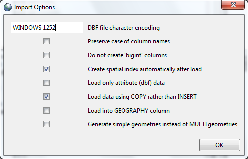
Under Plugins > PostGIS Shapefile and DBF Loader, Check the Options Menu. There are often problems when dealing with UTF-8 encoding in DBF files and when working in an MS Windows environment. Change encoding from UTF-8 to WINDOWS-1252 (another possibility would be LATIN-1). Keep boxes for creating spatial index and using COPY instead of INSERT checked.

Load

Browse and select both shapefiles. Once they appear in the import list the following elements must be changed: switch schema from public to desired schema (usa_general), change table to give each one a meaningful name, and specify the SRID number for each (since these files are from the US Census they’re in NAD 83, which is EPSG 4269). Once you hit Load, the log window will display the results of each import.

Refresh the database and both shapefiles will appear as tables.

Check Geometries

Because of the size of some geometries, they may appear blank if you preview the tables in pgAdmin – this is a well known and documented issue. The simplest way to verify is to check and make sure that none of the geometry columns are null:

SELECT COUNT(*)
FROM usa_general.states
WHERE geom IS NULL;

“0”

Post-Load Operations

Primary Keys

By default, PostGIS will automatically create a field called gid using sequential integers, and will designate this field as the primary key. If the data already has a natural key that you want to use, you would have to drop the key constraint on gid and add the constraint to the desired field. Since features from the US Census have unique ANSI / FIPS codes, we’ll designate that as the key.

ALTER TABLE usa_general.states
DROP CONSTRAINT states_pkey

Query returned successfully with no result in 125 ms.

ALTER TABLE usa_general.states
ADD CONSTRAINT states_pkey PRIMARY KEY (“state”);

Query returned successfully with no result in 125 ms.

Constraints

An alternative to changing the primary key would be to add UNIQUE and NOT NULL constraints to additional columns; gid remains as the primary key but the other columns will automatically be indexed when constraints are added.

ALTER TABLE usa_general.metros ADD CONSTRAINT cbsa_unq UNIQUE (cbsa);
ALTER TABLE usa_general.metros ALTER COLUMN cbsa SET NOT NULL;

Delete Records

For sake of example, we’ll delete all the records for micropolitan areas in the metros table, so we’re left with just metropolitan areas.

DELETE FROM usa_general.metros
WHERE lsad=’Micro’

Query returned successfully: 581 rows affected, 219 ms execution time.

Spatial SQL

As a test we can do a query to select all of the populated places that are within the NYC metropolitan area but are not in Pennsylvania, that have an elevation greater than or equal to 500 feet.

SELECT feature_name, state_alpha, county_name, elev_in_ft
FROM usa_general.pop_places, usa_general.metros
WHERE metros.cbsa=’35620′
AND ST_WITHIN(pop_places.geom, metros.geom)
AND elev_in_ft >= 500
AND state_alpha !=’PA’
ORDER BY elev_in_ft DESC

“Kampe”;”NJ”;”Sussex”;1293
“Highland Lakes”;”NJ”;”Sussex”;1283
“Edison”;”NJ”;”Sussex”;1234″…

Connect to QGIS

We can look at the geographic features by establishing a connection between the database and QGIS. In QGIS we can either hit the add PostGIS Layer button or use the browser to connect to a our database; we need to add the connection name, host, port, and database name. The username and password can be left blank and Q will prompt the user for it (if you don’t want it saved on the system). Once the connection is established you can add the layers to the view and change the symbolization.

I started out using QGIS to create my mapset and to connect it to my SQLite db which I had created and loaded with some census data. Then I thought, why not give the GRASS interface a try? I started using the newer Python-wx GUI and as I’m trying different things, I bounce back and forth between using the GUI for launching commands and the command line for typing them in – all the while I have Open Source GIS A GRASS GIS Approach at my side and the online manual a click away . So far, so good.

I loaded and cleaned a shapefile with the GRASS GUI (the GUI launches v.in.ogr, v.build, abd v.clean) and it’s attributes were loaded into the SQLite database I had set (using db.connect – need to do this otherwise a DBF is created by default for storing attributes). Then I had an age-old task to perform – the US Census FIPS / ANSI codes where stored in separate fields, and in order to join them to my attribute tables I had to concatenate them. I also needed to append some zeros to census tract IDs that lacked them – FIPS codes for states are two digits long, counties are three digits, and tracts are between four and six digits, but to standardize them four digit tracts should have two zeros appended.

Added the new JOIN_ID column using v.db.addcol, then did the following using db.execute:

UPDATE tracts_us99_nad83
SET JOIN_ID = STATE || COUNTY || TRACT

Then:

UPDATE tracts_us99_nad83
SET JOIN_ID = JOIN_ID || ’00’
WHERE length(JOIN_ID)=9

So this:

STATE COUNTY TRACT
01 077 0113
01 077 0114
01 077 011502
01 077 011602

Becomes this:

JOIN_ID
01077011300
01077011400
01077011502
01077011602

I could have done this a few different ways from within GRASS: instead of the separate v.db.addcol command I could have written a SQL statement in db.execute to alter the table and add a column. Or, instead of db.execute I could have used the v.db.update command.

My plan is to use GRASS for geoprocessing and analysis (will be doing some buffering, geographic selection, and basic spatial stats), and QGIS for displaying and creating final maps. I just used v.in.db to transform an attribute table with coordinates in my db to a point vector. But now I’m realizing that in order to draw buffers, I’ll need a projected coordinate system that uses meters or feet, as inputting degrees for a buffer distance (for points throughout the US) isn’t going to work too well. I’m also having trouble figuring out how to link my attribute data to my vectors – I can easily use v.db.join to fuse the two together, but there is a way to link them more loosely using the CAT ID number for each vector, but I’m getting stuck. We’ll see how it goes.

Some final notes – since I’m working with large datasets (every census tract in the US) and GRASS uses a topological data model where common node and boundaries between polygons are shared, geoprocessing can take awhile. I’ve gotten in the habit of testing things out on a small subset of my vectors, and once I get it right I run the process on the total set.

Lastly, there are times where I read about commands in the manual and for the life of me I can’t find them in the GUI – for example, finding a menu to delete (i.e. permanently remove) layers. But if you type the command without any of its parameters in the command line (in this case, g.remove) it will launch the right window in the GUI.

Another possibility is to dump DBF all together; even though the join table option in the fTools menu in QGIS only presents you the option of joining shapfiles or DBF, it turns out if you choose the DBF radio button option you can actually point to DBFs OR CSV files when you’re browsing to point to your data table. The join proceeds the same way, and you get a new shapefile with the data from the CSV joined to it. CSVs can be easily created from any spreadsheet, text editor, or database program in any operating system, so you can prep your attribute data in your program of choice before exporting to CSV and importing to GIS.

The problem with this approach is that all of the fields from the CSV file are automatically saved as text or strings when they’re appended to the shapefile. This means that any numeric data you have can’t be treated numerically; you can’t perform calculations or classify data as value ranges for mapping. You can go into the attribute table, enter the edit mode, and use the field calculator to create new fields where you convert the values to integers, but this adds a bunch of duplicate fields and is rather messy. You can’t delete columns from shapefiles within QGIS; you have to edit the attributes outside the software to remove extra columns.

Here’s an easy work around: you can create a CSVT file to go along with your CSV file. Open a text editor like Notepad or gedit and create a one line file where you specify the data type for each of the fields in your CSV file. Save the CSVT with the SAME NAME as your CSV file. Now when you go to join your CSV to your shapefile in QGIS, it will read the CSVT and save all of your fields properly in the new shapefile.

So for a CSV file like this with six fields:

CODE, ST, ID_NAICS51, EMP_51, ID_TOTAL, TOTAL_EMP
01, AL, ENU0100010551, 27013, ENU0100010510, 1570188
02, AK, ENU0200010551, 6988, ENU0200010510, 237708
04, AZ, ENU 0400010551, 41833, ENU0400010510, 2174919 …

You’d create a CSVT file like this:

“String”, “String”, “String”, “Integer”, “String”, “Integer”

So the 4th and 6th fields that have numeric values are saved as integers. There are a few other field types you can use, like Real for decimal numbers and some Date / Time options, and you can specify length and precision – see this post for details.

Using shapefiles, CSVs, and CSVTs are fine for small to medium projects and for the introductory workshops I’m teaching; geodatabases are another option and are certainly better for medium to large projects, but introducing them in my intro workshop is a little too much.

(NOTE – in QGIS 1.7 the join tool has been dropped from the ftools menu. To join a csv or dbf in 1.7+, you have to add your data table as a vector to your map, and then use the join tab within the properties menu of the feature you want to join it to. See this post for details.)

Fire up the GUI, and create a new, empty geodatabase under the File menu.Once we have a container, we can hit the load a shapefile button. I have a census PUMA layer for NYC that I’ve formatted by erasing water features. Click load, go to the path, give the file a nice brief name, and specify the SRID – the EPSG code that specifies what coordinate system my shapefile is in. In this case, it’s 4269 as the layer is in NAD83 (you can check your files by opening the prj file in a text editor or by using the OGR tools).

Once it’s loaded, you can expand the listing in the table of contents to see all the field names of the feature, and you can right click on it and choose the edit option to see all of the data in the attribute table.

Next we can load a data table. I have a 2006-2008 ACS census table in tab-delimited text format that I’ve pre-formatted. The table has the number of workers (labor force age 16+) and number of workers who commuted to work via the subway for every PUMA in the State of New York (it’s faster to download the whole state and filter out the city PUMAs later). Hit the load txt/csv button, specify a path, a new table name (subway_commuters), the delimiter used, and load the table. It’s given a different icon in the table of contents (toc), to distinguish a regular data table from a feature class.

The next step is to join them together; I already insured that they both share a common, unique identifier; a FIPS code that has a state and PUMA code. If I run a standard SELECT query I can join the tables in a temporary view – but that’s not what I want. I can save the query as a view, but I won’t be able to access the view within QGIS (at least not with this current stable version of SpatialLite, 2.31). What we have to do here is create a brand new table that combines both the puma feature class and the subway commuter table (referred to in Microsoft Access land as a Make Table Query). Here’s the SQL that we type in the command window:

CREATE TABLE pumas_nyc_subcom AS
SELECT *
FROM nyc_pumas, sub_commuters
WHERE PUMA5ID00=GEO_ID2

Execute the query, and we get a message that an empty results set was generated. Uh, ok. But then if we select the database path at the top of the TOC , right-click, and refresh, we’ll see our new combined table, pumas_nyc_subcom, and we can expand it and take a look at the data. The join worked, but we’re not done yet. Right now this is just a regular old data table (notice the icon?) We have to turn this into a feature class next.

Expand the fields for the new table in the TOC, select the Geometry field, right click, and check the geometry. We’ll see that it’s MULTIPOLYGON geometry, the projection is still NAD83, and there are 55 features (the non-NYC PUMAS were filtered out during the join, leaving us just with NYC data). Right click on Geometry again, choose the option to Recover Geometry. Specify the geometry type and the SRID, run, refresh the database, and success. A little globe appears next to pumas_nyc_subcom, indicating that it’s now a feature class.

At this point we can fire up QGIS. In the toolbar for versions post 1.02, there should be a connect to SpatialLite button. Hit connect, add a New database, and browse to get to it. Once it’s loaded, then we can hit connect to connect to it, and we’ll be able to see all feature classes (but NOT data tables, which is why we had to go through the join). Select pumas_nyc_subcom, which has features and data, and click add.

As with any GIS, now we have to symbolize the features to map the subway commuters. Right click on the layer in the table of contents, select properties, and you’ll get to the recently redesigned properties menu. Go to Symbology, map the subway commuters field by graduated values, change some colors, and voila, a map!

The developers are still experimenting with improvements – there’s a button in the upper right-hand corner of the symbology tab that asks you if you want to try the New Symbology – this is a new layout, with the introduction of graduated color palettes. It’s pretty slick, but still a work in progress (color ranges are assigned from dark to light, with the lowest values getting the darkest color; the opposite of cartographic convention). The same label properties are there too, but you can experiment with the improved labeling engine under the Plugins menu. The automatic placement of labels is vastly improved.

Mapping totals for subway commuters isn’t as interesting as mapping the percentage of commuters in each PUMA who ride the subway. So I’ll share my experiments working with calculated fields (in SpatialLite and QGIS) in my next post.

Whenever you create new features in a shapefile, ArcGIS automatically adds a couple of fields, including an auto-number ID field that uniquely identifies each feature. This was sufficient for our example as the 291 place names we were working with do not have a standard ID number that represents them. If we were creating features that did have a recognized ID number or code, we certainly would want to add an additional field to hold that number. This would allow us to share and relate our data to other datasets that use that conventional ID. For example, if we had a layer with the 50 states, we would want to have a FIPS number or the two digit postal code for each state in the attribute table, so we could relate our states feature to the zillions of other state-based data tables out there that also use these codes.

It’s also helpful to add other identifiers to relate our place names to some larger geographic area. Why? Let’s say we want to filter our neighborhoods by borough – perhaps we just want to label neighborhoods in Manhattan or calculate distances only between places that appear in the Bronx. It would be useful to have a borough code or some other code associated with each of our place names for running queries.

As it turns out, the City of New York does use a standardized system of three digit codes to identify all boroughs and community districts in the city. In our example, the code for Manhattan Community District 12, which contains Inwood and Washington Heights, is 112. The first digit identifies the borugh and the second two digits identify the district. It would be a good idea to assign each of our neighborhoods this district code, so we could filter our features by either borough or district.

When we create each feature, we could manually type in the code in it’s own field just like we added the neighborhood names, but that would be rather tedious – and unnecessary. A better choice would be to do a spatial join. Whereas a “regular” join allows us to join attribute tables based on a common ID field, a spatial join allows us to assign attributes to one layer based on their geographical relationship to another layer.

In the Table of Contents, right click on the neighborhoods layer and choose Joins and Relates – Joins. We’ll get the familiar Join dialog box. However, if you hit the first drop down box that says Join Attributes From a Table and choose Join Data Based on Spatial Location, we’ll get the options for doing a spatial join. Choose the community districts as the layer to join to the neighborhoods, and since we’re joining points to polygons we’ll choose parameters that are relevant for relating these two features. In this case, give each point (neighborhood / place) the attributes of the polygons (districts) that it falls inside. ArcGIS will create a new point layer with the joined fields when you hit OK. Open the attribute table of the new point layer, and you’ll see the additional fields, including the community district numbers. You’ll also get some rather useless fields from the district layer, like the length and area of each district, which you can safely delete.

So instead of tediously entering these numbers by hand for each neighborhood, we simply run the spatial join process once (after we’ve finished adding the points for all 291 neighborhoods) and the IDs are automatically added.

These points will be used for labeling each neighborhood. In this case, creating a new, georeferenced layer is preferable to creating 291 text labels on a map that are not tied to geography in any way.

• The first step is to download some layers from the NYC Department of Planning to use for reference, such as a layer for boroughs and community districts. Community districts are used by the city to approximate neighborhoods. Many of the neighborhoods that we are trying to plot are, in many cases, smaller areas or places within these boundaries.

• Next, open ArcCatalog and create a folder to store the data. Then, right click on the folder in the table of contents and select New – Shapefile. In the Create New Shapefile window, we give the shapefile a name, select Point as the feature type, and hit Edit to change the
  coordinate system. In the Spatial Reference Properties menu, we’ll import a coordinate system from one of the files we downloaded from NYC Planning, which uses New York State Plane for Long Island. Click OK and OK again, and we’ll have a new shapefile.

• Right now, our new shapefile isn’t very exciting because it’s empty – you can preview it in the catalog to see for yourself. If you preview the table, you’ll see that Arc created three fields – FID, Shape, and ID, which it will automatically fill in when we start creating features. Before we do that, we’ll have to add an additional column to store the name of the neighborhood. To do that, open ArcMap and add the neighborhood layer to the map. Then, right click on the layer in the Table of Contents and open the attribute table. Hit the Options button and choose Add Field. In the Add Field menu, name the new field, choose Text as the type, and change the length to 80 (in case we have some neighborhoods with long names). Hit OK, and you’ll have a new field.

• Let’s add our reference layers next. Hit the Add Data button (or File – Add Data), and add the borough boundaries and community districts (if you don’t see anything after you add them, right click on one of these layers and choose Zoom to Layer). Go into the symbology tab for each layer and change their display to make the areas appear more distinctive. Make sure your neighborhood layer is on top of your other layers.

• Now it’s time to start plotting neighborhoods. Go to the Selection menu – Set selectable Layers, and turn off all the layers except the neighborhood layer. Then, use the dropdown on the Editor Toolbar and Select Start Editing (if you don’t see the Editor Toolbar, make sure it’s activated by going to View – Toolbars and select it). On the Editor Toolbar, make sure the Create New Feature task is activated and that the target layer is the neighborhood layer, and not any of the reference layers. Zoom in to the top of Manhattan. With the Pencil tool selected in the toolbar, and using your sources (NYC planning map, Rand McNally street map, whatever), click on the map to approximate where the center of the Inwood neighborhood would be. A blue dot should appear on the map. Then right-click on the neighborhoods layer in the Table of Contents and open the attributes table. You’ll see a brand new record for your new dot. Click in the empty field for Name, type in the name of the neighborhood, and press enter.

• That’s the process! Next, locate the area for Washington Heights and click on the map to create the point for that neighborhood. The new dot will appear hi-lighted, while the previous dot for Inwood will now appear as a regular point symbol. Now it’s just a matter of plugging away. Make sure to occasionally save your edits by clicking Editor and choosing Save Edits. If you make a mistake, you can delete a feature by selecting the Select Feature tool in the regular tool bar (white arrow with a blue and white feature box next to it), select the particular point, and hit the delete key. If you’re having trouble pinpointing the right location for the neighborhood, try downloading additional reference layers to guide you. The NYC DOITT also has a page with GIS layers for the city with features like parks and streets that may be helpful. When you’re finished editing, choose Stop Editing under the Editor Toolbar.

• The ultimate goal of this exercise was to get neighborhood labels to appear without the actual point. To accomplish this, change the point symbol for the neighborhood to nothing by going into the Symbology tab for the layer and reducing the fill to no color, the outline to nothing, and the size to zero. Then open the Labels tab under the Properties menu, turn labels on using the name field as the label field, select Placement Properties and choose the setting to place the labels on top of the point, hit ok, and voila! Perfectly centered neighborhood names that are part of a georeferenced layer.

This covers the basics. In the next post, I’ll go a little further and discuss adding additional fields to the new file, without having to type them in manually.