Loading shapefiles can be done via the pgAdmin III GUI (for this example, used version 1.18 for MS Windows) from a client machine using the shp2pgsql-gui. This is an extra plugin that must be downloaded and installed. A command line version of the tool (shp2pgsql) is automatically bundled with PostGIS, but can’t be used by a client unless they either log into the server via a terminal or install PostGIS locally.

Download Plugin

The shp2pgsql-gui can be downloaded for MS Windows from the extras folder on the PostGIS website: http://download.osgeo.org/postgis/windows/. Version 2.01 for 32 bit environment was downloaded and unzipped. Per the instructions in the README file, the postgisgui folder was dragged into the PG BIN path as designated in pgAdmin under File > Options > Binary Paths. Once pgAdmin was restarted the gui was available under the Plugins menu.

Load Shapefiles

Set Options

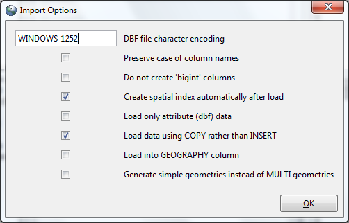
Under Plugins > PostGIS Shapefile and DBF Loader, Check the Options Menu. There are often problems when dealing with UTF-8 encoding in DBF files and when working in an MS Windows environment. Change encoding from UTF-8 to WINDOWS-1252 (another possibility would be LATIN-1). Keep boxes for creating spatial index and using COPY instead of INSERT checked.

Load

Browse and select both shapefiles. Once they appear in the import list the following elements must be changed: switch schema from public to desired schema (usa_general), change table to give each one a meaningful name, and specify the SRID number for each (since these files are from the US Census they’re in NAD 83, which is EPSG 4269). Once you hit Load, the log window will display the results of each import.

Refresh the database and both shapefiles will appear as tables.

Check Geometries

Because of the size of some geometries, they may appear blank if you preview the tables in pgAdmin – this is a well known and documented issue. The simplest way to verify is to check and make sure that none of the geometry columns are null:

SELECT COUNT(*)
FROM usa_general.states
WHERE geom IS NULL;

“0”

Post-Load Operations

Primary Keys

By default, PostGIS will automatically create a field called gid using sequential integers, and will designate this field as the primary key. If the data already has a natural key that you want to use, you would have to drop the key constraint on gid and add the constraint to the desired field. Since features from the US Census have unique ANSI / FIPS codes, we’ll designate that as the key.

ALTER TABLE usa_general.states
DROP CONSTRAINT states_pkey

Query returned successfully with no result in 125 ms.

ALTER TABLE usa_general.states
ADD CONSTRAINT states_pkey PRIMARY KEY (“state”);

Query returned successfully with no result in 125 ms.

Constraints

An alternative to changing the primary key would be to add UNIQUE and NOT NULL constraints to additional columns; gid remains as the primary key but the other columns will automatically be indexed when constraints are added.

ALTER TABLE usa_general.metros ADD CONSTRAINT cbsa_unq UNIQUE (cbsa);
ALTER TABLE usa_general.metros ALTER COLUMN cbsa SET NOT NULL;

Delete Records

For sake of example, we’ll delete all the records for micropolitan areas in the metros table, so we’re left with just metropolitan areas.

DELETE FROM usa_general.metros
WHERE lsad=’Micro’

Query returned successfully: 581 rows affected, 219 ms execution time.

Spatial SQL

As a test we can do a query to select all of the populated places that are within the NYC metropolitan area but are not in Pennsylvania, that have an elevation greater than or equal to 500 feet.

SELECT feature_name, state_alpha, county_name, elev_in_ft
FROM usa_general.pop_places, usa_general.metros
WHERE metros.cbsa=’35620′
AND ST_WITHIN(pop_places.geom, metros.geom)
AND elev_in_ft >= 500
AND state_alpha !=’PA’
ORDER BY elev_in_ft DESC

“Kampe”;”NJ”;”Sussex”;1293
“Highland Lakes”;”NJ”;”Sussex”;1283
“Edison”;”NJ”;”Sussex”;1234″…

Connect to QGIS

We can look at the geographic features by establishing a connection between the database and QGIS. In QGIS we can either hit the add PostGIS Layer button or use the browser to connect to a our database; we need to add the connection name, host, port, and database name. The username and password can be left blank and Q will prompt the user for it (if you don’t want it saved on the system). Once the connection is established you can add the layers to the view and change the symbolization.

I’m working with a developer who’s installed and configured the database on a server, and I’m accessing it remotely using pgAdmin. I’ve started loading data and running queries and so far I’m relieved that most of what I’m seeing seems familiar, having worked with SQLite / Spatialite for a few years now. I’m using the excellent book PostGIS in Action as my guide. Here’s my take on loading a text file with coordinates into the db and building geometry for it. Loading shapefiles, spatial SQL experiments, and connecting to Geoserver will follow.

Verify Version

SELECT postgis_full_version();

“POSTGIS=”2.1.1 r12113″ GEOS=”3.4.2-CAPI-1.8.2 r3921″ PROJ=”Rel. 4.8.0, 6 March 2012″ GDAL=”GDAL 1.9.2, released 2012/10/08″ LIBXML=”2.7.6″ LIBJSON=”UNKNOWN” TOPOLOGY RASTER”

Create Schema for Holding Related Objects

CREATE SCHEMA usa_general;

Query returned successfully with no result in 297 ms.

Import Delimited Text File

Test file is the US Populated Places gazetteer file from the USGS Geographic Names Information Service (GNIS). It is a pipe-delimited text file in encoded in UTF-8 with longitude and latitude coordinates in both DMS and DEC format. http://geonames.usgs.gov/domestic/download_data.htm

Create Table for Holding Data

CREATE TABLE usa_general.pop_places
(
feature_id int NOT NULL PRIMARY KEY,
feature_name varchar,
feature_class varchar,
state_alpha char(2),
state_numeric char(2),
county_name varchar,
county_numeric char(3),
primary_lat_dms varchar,
prim_long_dms varchar,
prim_lat_dec float4,
prim_long_dec float4,
source_lat_dms varchar,
source_long_dms varchar,
source_lat_dec float4,
source_long_dec float4,
elev_in_m int,
elev_in_ft int,
map_name varchar,
date_created date,
date_edited date
);

Query returned successfully with no result in 390 ms.

Copy Data From File

Must be run from the PSQL Console plugin in order to load data from a local client machine. If data was stored on the server, you could use the PGAdmin GUI and use COPY in an SQL statement instead of \copy. When running the PSQL Console on MS Windows the default character encoding is WIN1252. In this example, the data contains characters unsupported by this encoding; the file is encoded in UTF-8 and the console must be set to match. COPY is not a standard SQL command but is native to PostgreSQL.

— The optional HEADER specifies that the data file has a header column that should be skipped when importing

\encoding UTF8
\copy usa_general.pop_places
FROM ‘C:\Workspace\postgis_testing\POP_PLACES_20140204.txt’
DELIMITER ‘|’ CSV HEADER

Basic Query to Test that Load was Success

SELECT *
FROM usa_general.pop_places
WHERE state_alpha=’NY’ and county_name=’New York’
ORDER BY feature_name

Create Geometry from Coordinates and Make Spatial Index

4269 is the EPSG code for NAD 83, the basic geographic coordinate system used by US government agencies.

SELECT AddGeometryColumn(‘usa_general’,’pop_places’,’geom’,4269,’POINT’,2)

“usa_general.pop_places.geom SRID:4269 TYPE:POINT DIMS:2 ”

UPDATE usa_general.pop_places
SET geom = ST_GeomFromText(‘POINT(‘|| prim_long_dec || ‘ ‘|| prim_lat_dec || ‘)’,4269);

Query returned successfully: 200359 rows affected, 18268 ms execution time.

CREATE INDEX idx_pop_places_geom
ON usa_general.pop_places USING gist(geom);

Query returned successfully with no result in 8439 ms.

Basic SQL Query to Test Geometry

ST_AsEWKT transforms the output of geometry from binary code into the OGC Well Known Text format (WKT).

SELECT feature_name, ST_AsEWKT(geom) AS geometry
FROM usa_general.pop_places
WHERE state_alpha=’NY’ AND county_name=’New York’
ORDER BY feature_name

“Amalgamated Dwellings”;”SRID=4269;POINT(-73.9828 40.715)”
“Amsterdam Houses”;”SRID=4269;POINT(-73.9881 40.7731)”
“Battery Park City”;”SRID=4269;POINT(-74.0163 40.7115)”…

Basic Spatial SQL Query to Test Geometry

Selects the northernmost point in the table.

SELECT feature_name, state_alpha, ST_AsEWKT(geom) AS geometry
FROM usa_general.pop_places
WHERE ST_Xmax(geom) IN(
SELECT Max(ST_Xmax(geom))
FROM usa_general.pop_places)

“Amchitka”;”AK”;”SRID=4269;POINT(178.878 51.5672)”

Drop Columns

Drop some columns that have no data.

ALTER TABLE usa_general.pop_places
DROP COLUMN source_lat_dms,
DROP COLUMN source_long_dms,
DROP COLUMN source_lat_dec,
DROP COLUMN source_long_dec;

Query returned successfully with no result in 180 ms.

Users navigate via a web map (Google by default but you can choose other options), and as they change the extent by panning or zooming a list of available spatial layers appears in a table of contents beside the map. Hovering over a layer in the contents reveals a bounding box that indicates its spatial extent. Several algorithms determine the ranking order of the results based on the spatial intersection of bounding boxes with the current map view. For instance, layers that are completely contained in the map view have priority over those that aren’t, and layers that have their geographic center in the view are also pushed higher in the results. Non-spatial search filters for date, data type, institution, and keywords help narrow down a search. Of course, the quality of the results is completely dependent on the underlying metadata for the layers, which is stored in the various repositories.

The project was pioneered by Tufts, Harvard, and MIT , and now about a dozen other large research universities are actively working with it, and others are starting to experiment. The purpose of the summit was to begin creating a cohesive community to manage and govern the project, and to increase and outline the possibilities for collaborating across institutions. At the back end, librarians and metadata experts are loading layers and metadata into their repositories; metadata creation is an exacting and time-consuming process, but the OGP will allow institutions to share their metadata records in the hope of avoiding duplicated effort. The OGP also allows for the export of detailed spatial metadata from FGDC and ISO to MODS and MARC, so that records for the spatial layers can be exported to other content management systems and library catalogs.

The summit gave metadata experts the opportunity to discuss best practices for metadata creation and maintenance, in the hopes of providing a consistent pool of records that can be shared; it also gave software developers the chance to lay out their road map for how they’ll function as an open source project (the OGP community could look towards the GeoNetwork opensource project, a forerunner in spatial metadata and search that’s used in Europe and by many international organizations). Series of five-minute talks called Ignite sessions gave librarians and developers the ability to share the work they were doing at their institutions, either with OGP in particular or with metadata and spatial search in general, which sparked further discussion.

The outcome of all the governance, resource sharing, and best practices discussions are available on a series of pages dedicated to the summit, on the opengeoportal.org project website. You can also experiment with the OGP via http://geodata.tufts.edu/, Tuft’s gateway to their repository. As you search for data you can identify which repository the data is coming from (Tufts, Harvard, or MIT) based on the little icon that appears beside each layer name. Public datasets (like US census layers) can be downloaded by anyone, while copyrighted sets that the schools’ purchased for their users require authentication.

OGP is a simple yet elegant open source project that operates under OGC standards and is awesome for spatial search, but the real gem here is the community of people that are forming around it. I was blown away by the level of expertise, dedication, and over all professionalism that each of the librarians, information specialists, and software developers exuded, via the discussions and particularly by the examples of the work they were doing at their institutions. Beyond just creating software, this project is poised to enhance the quality and compatibility of spatial metadata to keep our growing pile of geospatial stuff find-able.

I had my first peer-reviewed journal article published, Evaluating open source GIS for libraries. After my initial exploration of open source GIS that I documented on this blog over a year and a half ago, I took a systematic approach to evaluating a number of software packages for thematic mapping. This article documents the tests and results and provides the requisite background on open source software, GIS, and how both are manifest in academic libraries. Given the lengthy process of academic publishing (the whole process began in Dec 2008 with my first test and ended in March 2010 with publication), some of my observations of individual software packages have changed with the release of bug fixes, new features, and new versions. Generally, individual software packages and open source GIS as a whole have improved during this short span of time, but my primary observations and the big picture still hold.

Title: Evaluating open source GIS for libraries
Author(s): Francis P. Donnelly
Journal: Library Hi Tech
Year: 2010 Volume: 28 Issue: 1 Page: 131 – 151
ISSN: 0737-8831
DOI: 10.1108/07378831011026742
Publisher: Emerald Group Publishing Limited

I’ve previously mentioned Steiniger and Bocher’s excellent article, An overview on current free open source desktop GIS developments in the International Journal of Geographic Information Science, which Steiniger has posted on his website. I recently discovered he’s written a second article with Hay entitled Free and Open Source Geographic Information Tools for Landscape Ecology in Ecological Informatics, which is also available there. The second article provides an in-depth look and great summary tables of landscape analysis applications for eight different open source GIS apps, focusing on advanced tools for researchers. In contrast, my article focuses on basic mapping capabilities for novice to intermediate users.

The other milestone is this blog – I just noticed that we’ve passed the two year mark. While there have only been a few public comments here and there, I have received a number of emails over the years with questions and comments and the number of visitors to the site has grown consistently from month to month. I’m glad that it’s been useful to so many people; it’s certainly been useful to me (as an extension to my feeble brain) and I’ll endeavor to keep it going. Thanks to everyone for your comments and feedback. Best – frank

• There is a project called Sextante, which is essentially an open source ArcToolbox for gvSIG. It adds a lot of geoprocessing and analysis functions and is pretty easy to install. There are 200 + tools in the box, but for some reason not all of them are active. I’m not sure why this is the case, but haven’t poked around much to find out.

• There are also a number of extra plugins for QGIS that are available through the QGIS wiki under PluginRepository; they include plugins that add more symbolization and that make table joins possible. Haven’t had a chance to try this yet either, but it sounds like these extras could make QGIS a lot more viable as a thematic mapping option.

• I found out about the QGIS plugins from this article, which offers a good overview of QGIS. The article also discusses one of the other shortcomings of open source GIS – the lack of a support for a simple, desktop geodatabase similar to the Microsoft Access personal geodatabases. PostGIS is certainly powerful and there has been a lot written about it, but a server based geodatabase is not always the best solution, particularly for small, stand-alone projects. There is a cool project called Spatiallite, where someone has created geographically enabled SQLite databases (which are small, stand alone dbs). You can export shapefiles to them, or simply view and edit the attributes in a shapefile via a virtual connection. Based on what I’ve looked at thus far, you can access SQlite databases directly in GRASS and when using GRASS datasets via QGIS, but I haven’t been able to connect to a SQlite db with the other software I’ve looked at – it’s just not supported yet.

• In researching open source GIS, I’ve looked at a book specifically on GRASS, Open Source GIS: A Grass Approach, as well as two books on web mapping (GIS for Web Developers: Adding ‘Where’ to Your Web Applications and Web Mapping Illustrated: Using Open Source GIS Toolkits)which cover GDAL and OGR, QGIS, GIS servers, PostGIS and PostgreSQL, and a few other tools. There is a book that’s recently been published that focusses specifically on Open Source Desktop GIS – Desktop GIS: Mapping the Planet with Open Source Tools. I pre-ordered a copy on Amazon that was supposed to ship in Mid September, but is now being delayed until late October. Based on the table of contents it looks pretty thorough and covers many of the choices I listed in my previous post, and I’m looking forward to its arrival.

• Price. A single, stand-alone copy of ArcView costs $1500. Not only is that prohibitively expensive for me, it’s impossible for students. Which means that students who are taking a GIS class have to use the software in a computer lab on campus to complete assignments. This is not always convenient for many students, and is particularly problematic where I work since we are primarily a commuter campus.

• License limitations. If you’re running Arc through a central license server, PCs have to be connected to the server through a hardwired connection – no wireless. Our library has a laptop checkout program for students which would give students an alternative to using a computer lab. But not being able to install the software on a laptop eliminates this possibility. It also makes it a pain for me to give presentations, as I always have to make sure that the room I’ll be presenting in has the software. My short term solution is to use an eval copy on a laptop. You can purchases USB keys that have the license info on them, but if you work in a large, complex academic or government setting, getting one can be a challenge. And every year we have to go through the process of getting the license renewed.

• Installation and Bugs. As Arc users know, installation can be time consuming, particularly since you can’t have two versions of Arc installed concurrently – you have to uninstall one before installing the new one. And how many service packs have been issued for version 9.2? Six. IT people love it when they have to install fixes in a dozen labs / classrooms in the middle of a semester, particularly when they have to do it 5 or 6 times a year. In reality, we skip several service packs and live with the bugs.

• Forced Obsolescence. This is particularly aggravating. Every year or two, we all have to go through the ritual of making an upgrade, which involves time consuming un-installation and installation. And you need to make sure that different branches of your organization that use GIS are on the same page, otherwise you’ll run into incompatibility issues (like when mxd files created in version  9.2 don’t work in 9.1).

• Cross platform. I run a linux box at home and occasionally would like to take my work with me. There are a number of students and faculty members at my school who are ardent Mac users. But ArcGIS runs only on Windows.

The open source alternatives are free, easy to install (usually), can be installed anywhere without restrictions, the software doesn’t expire, and upgrades are a rather simple affair. The obvious downside is that none of them have the power, scope, or usability that ArcGIS has. At least, not yet.